6.1 Event-Driven Simulation

This chapter under construction.

Simulate the motion of N colliding particles according to the laws of elastic collision using event-driven simulation. Such simulations are widely used in molecular dynamics (MD) to understand and predict properties of physical systems at the particle level. This includes the motion of molecules in a gas, the dynamics of chemical reactions, atomic diffusion, sphere packing, the stability of the rings around Saturn, the phase transitions of cerium and cesium, one-dimensional self-gravitating systems, and front propagation. The same techniques apply to other domains that involve physical modeling of particle systems including computer graphics, computer games, and robotics. We will revisit some of these issues again in Chapter 7.

a good reference

Hard sphere model. The hard sphere model (billiard ball model) is an idealized model of the motion of atoms or molecules in a container. We focus on the two-dimensional version called the hard disc model. The salient properties of this model are listed below.

N particles in motion, confined in the unit box.
Particle i has known position (rx_i, ry_i), velocity (vx_i, vy_i), mass m_i, and radius σ_i.
Particles interact via elastic collisions with each other and with the reflecting boundary.
No other forces are exerted. Thus, particles travel in straight lines at constant speed between collisions.

This simple model plays a central role in statistical mechanics, a field which relates macroscopic observables (e.g., temperature, pressure, diffusion constant) to microscopic dynamics (motion of individual atoms and molecules). Maxwell and Boltzmann used the model to derive the distribution of speeds of interacting molecules as a function of temperature; Einstein used it to explain the Brownian motion of pollen grains immersed in water.

Simulation. There are two natural approaches to simulating the system of particles.

Time-driven simulation. Discretize time into quanta of size dt. Update the position of each particle after every dt units of time and check for overlaps. If there is an overlap, roll back the clock to the time of the collision, update the velocities of the colliding particles, and continue the simulation. This approach is simple, but it suffers from two significant drawbacks. First, we must perform N² overlap checks per time quantum. Second, we may miss collisions if dt is too large and colliding particles fail to overlap when we are looking. To ensure a reasonably accurate simulation, we must choose dt to be very small, and this slows down the simulation.
Event-driven simulation. With event-driven simulation we focus only on those times at which interesting events occur. In the hard disc model, all particles travel in straight line trajectories at constant speeds between collisions. Thus, our main challenge is to determine the ordered sequence of particle collisions. We address this challenge by maintaining a priority queue of future events, ordered by time. At any given time, the priority queue contains all future collisions that would occur, assuming each particle moves in a straight line trajectory forever. As particles collide and change direction, some of the events scheduled on the priority queue become "stale" or "invalidated", and no longer correspond to physical collisions. We adopt a lazy strategy, leaving such invalidated collision on the priority queue, waiting to identify and discard them as they are deleted. The main event-driven simulation loop works as follows:
- Delete the impending event, i.e., the one with the minimum priority t.
- If the event corresponds to an invalidated collision, discard it. The event is invalid if one of the particles has participated in a collision since the time the event was inserted onto the priority queue.
- If the event corresponds to a physical collision between particles i and j:
  - Advance all particles to time t along a straight line trajectory.
  - Update the velocities of the two colliding particles i and j according to the laws of elastic collision.
  - Determine all future collisions that would occur involving either i or j, assuming all particles move in straight line trajectories from time t onwards. Insert these events onto the priority queue.
- If the event corresponds to a physical collision between particles i and a wall, do the analogous thing for particle i.
This event-driven approach results in a more robust, accurate, and efficient simulation than the time-driven one.

Collision prediction. We review the formulas that specify if and when a particle will collide with the boundary or with another particle, assuming all particles travel in straight-line trajectories.

Collision between particle and a wall. Given the position (rx, ry), velocity (vx, vy), and radius σ of a particle at time t, we wish to determine if and when it will collide with a vertical or horizontal wall.

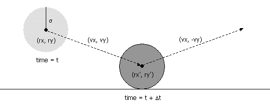
Since the coordinates are between 0 and 1, a particle comes into contact with a horizontal wall at time t + Δt if the quantity ry + Δt vy equals either σ or (1 - σ). Solving for Δt yields:

An analogous equation predicts the time of collision with a vertical wall.
Collision between two particles. Given the positions and velocities of two particles i and j at time t, we wish to determine if and when they will collide with each other.

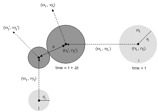
Let (rx_i' , ry_i' ) and (rx_j' , ry_j' ) denote the positions of particles i and j at the moment of contact, say t + Δt. When the particles collide, their centers are separated by a distance of σ = σ_i + σ_j. In other words:
σ² = (rx_i' - rx_j' )² + (ry_i' - ry_j' )²
During the time prior to the collision, the particles move in straight-line trajectories. Thus,
rx_i' = rx_i + Δt vx_i, ry_i' = ry_i + Δt vy_i
rx_j' = rx_j + Δt vx_j, ry_j' = ry_j + Δt vy_j
Substituting these four equations into the previous one, solving the resulting quadratic equation for Δt, selecting the physically relevant root, and simplifying, we obtain an expression for Δt in terms of the known positions, velocities, and radii.

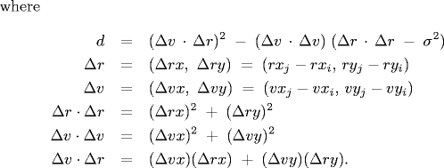
If either Δv ⋅ Δr ≥ 0 or d < 0, then the quadratic equation has no solution for Δt > 0; otherwise we are guaranteed that Δt ≥ 0.

Collision resolution. In this section we present the physical formulas that specify the behavior of a particle after an elastic collision with a reflecting boundary or with another particle. For simplicity, we ignore multi-particle collisions. There are three equations governing the elastic collision between a pair of hard discs: (i) conservation of linear momentum, (ii) conservation of kinetic energy, and (iii) upon collision, the normal force acts perpendicular to the surface at the collision point. Physics-ly inclined students are encouraged to derive the equations from first principles; the rest of you may keep reading.

Between particle and wall. If a particle with velocity (vx, vy) collides with a wall perpendicular to x-axis, then the new velocity is (-vx, vy); if it collides with a wall perpendicular to the y-axis, then the new velocity is (vx, -vy).
Between two particles. When two hard discs collide, the normal force acts along the line connecting their centers (assuming no friction or spin). The impulse (Jx, Jy) due to the normal force in the x and y directions of a perfectly elastic collision at the moment of contact is:

and where m_i and m_j are the masses of particles i and j, and σ, Δx, Δy and Δ v ⋅ Δr are defined as above. Once we know the impulse, we can apply Newton's second law (in momentum form) to compute the velocities immediately after the collision.
vx_i' = vx_i + Jx / m_i, vx_j' = vx_j - Jx / m_j
vy_i' = vy_i + Jy / m_i, vy_j' = vy_j - Jy / m_j

Particle collision simulation in Java. Our implementation involves the following data types: MinPQ.java, Particle.java, and CollisionSystem.java.

Particle data type. Represents particles moving in the unit box.
Event data type. Data type that represents collision events. There are four different types of events: a collision with a vertical wall, a collision with a horizontal wall, a collision between two particles, and a redraw event. This would be a fine opportunity to experiment with OOP and polymorphism. We propose the following simpler (but somewhat less elegant approach).
In order to implement isValid, the event data type should store the collision counts of the relevant particles at the time the event was created. The event corresponds to a physical collision if the current collision counts of the particles are still the same as when the event was created, i.e., no intervening collisions.

Data files. We use the following data format. The first line contains the number of particles N. Each of the remaining N lines consists of 6 real numbers (position, velocity, mass, and radius) followed by three integers (red, green, and blue values of color). You may assume that all of the position coordinates are between 0 and 1, and the color values are between 0 and 255. Also, you may assume that none of the particles intersect each other or the walls.

N                            
rx ry vx vy radius mass r g b
rx ry vx vy radius mass r g b
rx ry vx vy radius mass r g b
rx ry vx vy radius mass r g b

Here are some sample data files:

FILE	DESCRIPTION
p10.txt	10 particles
p2000.txt	2000 particles
diagonal.txt
diagonal1.txt
diagonal2.txt
wallbouncing.txt	9 particles in a row colliding with 9 particles in a column
wallbouncing2.txt	10 particles in a row not colliding with 9 particles in a column
wallbouncing3.txt	19 particles in a row colliding with 19 particles in a column
p100-.125K.txt	100 particles at 0.125 Kelvin
p100-.5K.txt	100 particles at 0.5 Kelvin
p100-2K.txt	100 particles at 2.0 Kelvin
p1000-.5K.txt	1000 particles at 0.5 Kelvin
p1000-2K.txt	1000 particles at 2.0 Kelvin
billiards2.txt	cue ball striking pyramid of 3 balls
billiards4.txt	cue ball striking pyramid of 10 balls
billiards5.txt	cue ball striking pyramid of 15 balls
diffusion.txt	diffusion of particles from one side of slit
diffusion2.txt	diffusion of particles from one quarter
diffusion3.txt
brownian.txt
brownian2.txt
squeeze.txt	one tiny particle sandwiched between two big particles
squeeze2.txt	one tiny particle sandwiched between two big particles
pendulum.txt	pendulum effect

Other potential data files

One particle in motion.
Two particles in head on collision.
Two particles, one at rest, colliding at an angle.
One red particle in motion, N blue particles at rest.
N particles on a lattice with random initial directions (but same speed) so that the total kinetic energy is consistent with some fixed temperature T, and total linear momentum = 0. Have a different data set for different values of T.
Diffusion I: assign N very tiny particles of the same size near the center of the container with random velocities.
Diffusion II: N blue particles on left, N green particles on right assigned velocities so that they are thermalized (e.g., leave partition between them and save positions and velocities after a while). Watch them mix. Calculate average diffusion rate?
N big particles so there isn't much room to move without hitting something.
Einstein's explanation of Brownian motion: 1 big red particle in the center, N smaller blue particles.

Exercises

Particle collision game. Implement the game Particles: you control a red ball with a mouse, trying to avoid colliding with blue balls that behave according to the laws of elastic collision. After a certain interval of time, introduce a new blue ball at random.
Brownian motion. In 1827, the botanist Robert Brown observed the motion of wildflower pollen grains immersed in water using a microscope. He observed that the pollen grains were in a random motion, following what would become known as Brownian motion. This phenomenon was discussed, but no convincing explanation was provided until Einstein provided a mathematical one in 1905. Einstein's explanation: the motion of the pollen grain particles was caused by millions of tiny molecules colliding with the larger particles. He gave detailed formulas describing the behavior of tiny particles suspended in a liquid at a given temperature. Einstein's explanation was intended to help justify the existence of atoms and molecules and could be used to estimate the size of the molecules. Einstein's theory of Brownian motion enables engineers to compute the diffusion constants of alloys by observing the motion of individual particles. Here's a demo of Einstein's explanation of Brownian motion from here.
Free path and free time. Free path = distance a particle travels between collisions. Plot histogram. Mean free path = average free path length over all particles. As temperature increases, mean free path increases (holding pressure constant). Compute free time length = time elapsed before a particle collides with another particle or wall.
Collision frequency. Number of collisions per second.
Root mean-square velocity. Root mean-square velocity / mean free path = collision frequency. Root mean square velocity = sqrt(3RT/M) where molar gas constant R = 8.314 J / mol K, T = temperature (e.g., 298.15 K), M = molecular mass (e.g., 0.0319998 kg for oxygen).
Maxwell-Boltzmann distribution. Distribution of velocity of particles in hard sphere model obey Maxwell-Boltzmann distribution (assuming system has thermalized and particles are sufficiently heavy that we can discount quantum-mechanical effects). Distribution shape depends on temperature. Velocity of each component has distribution proportional to exp(-mv_x^2 / 2kT). Magnitude of velocity in d dimensions has distribution proportional to v^(d-1) exp(-mv^2 / 2kT). Used in statistical mechanics because it is unwieldy to simulate on the order of 10^23 particles. Reason: velocity in x, y, and z directions are normal (if all particles have same mass and radius). In 2d, Rayleigh instead of Maxwell-Boltzmann.
Pressure. Main thermodynamic property of interest = mean pressure. Pressure = force per unit area exerted against container by colliding molecules. In 2d, pressure = average force per unit length on the wall of the container.
Temperature. Plot temperature over time (should be constant) = 1/N sum(mv^2) / (d k), where d = dimension = 2, k = Boltzmann's constant.
Diffusion. Molecules travel very quickly (faster than a speeding jet) but diffuse slowly because they collide with other molecules, thereby changing their direction. Two vessels connected by a pipe containing two different types of particles. Measure fraction of particles of each type in each vessel as a function of time.
Time reversibility. Change all velocities and run system backwards. Neglecting roundoff error, the system will return to its original state!
Maxwell's demon. Maxwell's demon is a thought experiment conjured up by James Clerk Maxwell in 1871 to contradict the second law of thermodynamics. Vertical wall in middle with molecule size trap door, N particles on left half and N on right half, particle can only go through trap door if demon lets it through. Demon lets through faster than average particles from left to right, and slower than average particles from right to left. Can use redistribution of energy to run a heat engine by allowing heat to flow from left to right. (Doesn't violate law because demon must interact with the physical world to observe the molecules. Demon must store information about which side of the trap door the molecule is on. Demon eventually runs out of storage space and must begin erasing previous accumulated information to make room for new information. This erasing of information increases the entropy, requiring kT ln 2 units of work.)
Metric space. Extend to support spheres and hyperplanes in an arbitrary metric space.
Cell method. Useful optimization: divide region into rectangular cells. Ensure that particles can only collide with particles in one of 9 adjacent cells in any time quantum. Reduces number of binary collision events that must be calculated. Downside: must monitor particles as they move from cell to cell.
Multi-particle collisions. Handle multi-particle collisions. Such collisions are important when simulating the break in a game of billiards.
Kinetic heaps or kinetic data structures. (Guibas)

6.1 Event-Driven Simulation

Exercises

Creative Exercises